Saturday 20 December 2014

Medical Image Analysis IPython Tutorials

As the Christmas break approaches and the Autumn term will soon be over, I am glad that I've been given the opportunity to feature on this blog the teaching material for the course Medical Image Computing that was newly introduced this year at Imperial College. This course, taught by Prof. Daniel Rueckert and Dr. Ben Glocker, aims to provide MSc students with the necessary skills to carry out research in medical image computing: visualisation, image processing, registration, segmentation and machine learning. The lectures were accompanied by tutorials in the form of IPython notebooks developped by Ozan Oktay, using SimpleITK to process medical images in Python and scikit-learn for Machine Learning. These tutorials are made available on github. They provide an introduction to medical imaging in Python that complements SimpleITK's official notebooks.

There are 4 tutorials:
  1. Basic manipulation of medical image, image filtering, contrast enhancement, and visualisation
  2. Image registration, multi-modal registration, Procrustes analysis
  3. EM segmentation and gaussian mixtures models, atlas prior, Otsu thresholding
  4. Machine learning: classification, regression and PCA.

Image registration is the process of aligning images (rigid registration) and warping them (non-rigid registration) in order to compare or combine images. A typical application is a patient being scanned twice at a few months interval and the two scans are registered in order to assess the evolution of a disease. Another application illustrated below (see tutorial 2) is a patient having an MRI and a CT scan, each modality highlighting different characteristics of a patient's anatomy, and a registration process is required before the doctors can overlay both images.

Image registration:
the CT scan (red) and the MRI scan (green) are registered in order to be combined in a single image.

Wednesday 12 November 2014

Viewing medical images in an IPython notebook

I was looking for a simple way to browse medical images within an IPython notebook, and came across the interact function which makes it really easy to work with sliders. The function irtk.imshow returns three orthogonal slices for a given (z,y,x) concatenated in a single image. PIL is used to avoid writing temporary images to disk.


In [1]:
import irtk

patient_id = '2159'
img = irtk.imread( patient_id + "_img.nii.gz" )
seg = irtk.imread( patient_id + "_seg.nii.gz" )
In [2]:
from IPython.html.widgets import interact, interactive, fixed
from IPython.html import widgets
from IPython.display import display

def f(z,y,x):
    display( irtk.imshow(img,seg,index=(z,y,x)) )
 
interact( f,
         z=widgets.IntSliderWidget(min=0,max=img.shape[0]-1,step=1,value=img.shape[0]/2),
         y=widgets.IntSliderWidget(min=0,max=img.shape[1]-1,step=1,value=img.shape[1]/2),
         x=widgets.IntSliderWidget(min=0,max=img.shape[2]-1,step=1,value=img.shape[2]/2) )


The sliders disappear when the notebook is saved as HTML, here are some hints for preserving the interactivity through JavaScript (though this is probably not the best approach for an image viewer).

Ideally, a medical image viewer integrated within the IPython notebook would use XTK, but there is still works to be done before it provides a working solution, see github/fperez and github/richstoner for proofs of concept.


Tuesday 21 October 2014

Creating a video from PDF slides with ffmpeg and ImageMagick

To illustrate the role of autocontext in [1], I created a video from the successive probability maps obtained in the segmentation of the left ventricle in 3D echocardiography. This post is a quick overview of the bash and LaTeX code I used for this video. The XKCD style for beamer is presented in a previous blog post.


The slides are first converted from PDF to PNG using ImageMagick, then each slide is transformed into a single movie in order to easily control the time spent on each frame (-t option of ffmpeg), as well as the insertion of other movies.

Monday 6 October 2014

Automated segmentation of the fetal brain in MRI

This summer, I had a paper accepted in NeuroImage [1] on a fully automated pipeline for motion correction of the fetal brain in MRI. My main contribution is on detecting the brain and extracting it in the unprocessed data in order to automatically provide an input for motion correction. The motion correction code is the work of Maria Murgasova [2], I incorporated in it the realignment of the slice segmentations in  order to refine the brain extraction throughout the motion correction process.

I recently installed the code on a new machine and tested it using the example on github. As installing research code is rarely a simple matter of downloading the source and running "make", I took notes of all the steps for future reference:

Wednesday 9 April 2014

Kaggle Galaxy Zoo: A Space Odyssey

During the last month, I took part in the Kaggle challenge on Galaxy Zoo. Kaggle is a platform for Machine Learning challenges, and the goal of the Galaxy Zoo challenge is to learn how humans classified galaxies in order to replace those humans by a program able to classify previously unseen galaxies. As my PhD is on the automated localisation of different fetal organs in MRI scans, Machine Learning is my current obsession (see my previous post on object detection). I chose to take part in this challenge out of my frustration of doing Machine Learning on 50 patients... Indeed, Galaxy Zoo lets us train on 61578 galaxies, and asks us to classify 79975 galaxies. As a result, after finishing 56th out of 329 participants (which puts me in the top 25%), it was an extremely fruitful experience.

I spoke of classification, but the annotations we actually learn from are the responses humans gave to a set of questions. Whereas most competitors went for a regression on the vector of all the human scores, I took a slightly different approach, learning features from the galaxies humans most agreed on.

I worked in Python, using OpenCV for cropping and rotating the galaxies, and scikit-learn for the machine learning part. I decided to use Random Forests (or the very similar Extremely Randomized Trees) to learn a regression on the whole traning data, thinking that if I managed to get the right features that could properly separate the data, it would work.

Thursday 27 March 2014

Object detection

This blog post aims to provide an overview of the main trends in object detection I encountered in the literature.

Object detection is the process of automatically detecting in an image instances of a class, such as cars or pedestrians. Object localisation is often considered synonym of detection, the main difference I see in medical imaging is that an MRI scan will contain one and only one heart or brain, a localisation task thus assumes the presence of the object in the image. However, in a typical computer vision task, an image could contain several cars or none at all, and the detection task must thus decide whether the object is present or not before finding its location in the image. In the following, I will talk indifferently of detection or localisation.

The simplest approach to find a given object in an image is template matching. This is a very limited approach deprived of any generalisation: it is principally aimed at finding the position of a cropped image in the original version of the image, but it can also be used for objects that have very little 
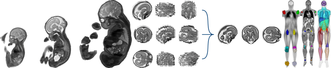
variation within a class. An example application in object detection is Anquez et al. (2009) who used template matching to detect the eyes of the fetus in motion free MRI scans, as a starting point for a brain detection pipeline.

In order to take into account the variable appearance of objects within a class, a machine learning framework is usually adopted. An algorithm is trained on training data, using validation data to tweak its various parameters. Testing data, which has not been seen by the detector during training or validation, is then used to assess the accuracy of the trained detector (Bradski et al., 2008). In order to make decisions about images, the algorithm extracts features, which can be as simple as the difference of mean intensities over two rectangular areas (Criminisi et al., 2011), or more complex such as histograms of SIFT features matched to their nearest neighbour in a “vocabulary” of image patches (Csurka et al., 2004). These features are then passed to a machine learning method such as Boosting, Random Forest or SVM, to learn the appearance of the object during training, or to make a decision at testing time. If you look at the common interface for feature detectors in OpenCV and the generic API for classifiers in scikit-learn, you shall notice that image features and machine learning methods are building blocks which can be easily interchanged. Switching between SIFT and SURF, or SVM and Random Forest can be as easy as changing a line of code. Among other things, the choice relies on a trade-off between the desired performance in speed or accuracy, whether your features need to be rotation invariant, the size of your training dataset, whether you have multi-channel images, your hardware limitations such as memory, and of course the implementations you have at hand. Independently of the choice of image features or machine learning method, the questions I am mostly interested for this blog post are the following:
  • At which positions in the image do you want to run your classifier? At every pixel, every superpixel or only on salient regions?
  • When your classifer is positioned in the image, is it voting for the current location or for an offset location (see Hough transform)?
  • Are you running only one detector, or a cascade of detectors? How do you then define “coarse to fine”?
  • If you need to detect several parts of an object, how do you take the spatial configuration into account instead of running independant detectors?
  • How do you summarize image information and combine different features?

Sunday 2 March 2014

XKCD-style beamer presentation (LaTeX)

Last December, I had a short presentation to do, not necessarily too formal, so I decided to have a go at the different XKCDify codes lying around the web to make a more original LaTeX beamer presentation.

It seems that a version of the code is now shipped with Matplotlib, with a basic example here, and the whole galery of Matplotlib examples turned into XKCD plots there.

I did not notice any official code back in December, from what I understood, the idea originated on the Matplotlib users mailing-list from Damon McDougall, followed by a blog post by Jake Vanderplas. But the code I finally used is from Johannes Buchner, with some hard-coded parameterisation. To simulate hand drawn lines with Tikz, I used the LaTex code from percusse.

For the font, I recommand the LaTeX font catalogue to avoid any installation trouble, but in the end, I used the script from Holger Widmann to install Humor-Sans.ttf, which can be downloaded from several places.

Lastly, some LaTeX code to use the font:
%% use xkcd font
%% Note: that's a font with no bold or italic...
\usepackage[T1]{fontenc}
\definecolor{xkcd_color}{rgb}{.376,.435,.533}
\usecolortheme[named=xkcd_color]{structure}
\renewcommand{\familydefault}{xkcd}

and some page layout changes for the Boadilla theme:
%% do not use any \useoutertheme{}

%% disable navigation symbols
\setbeamertemplate{navigation symbols}{}

%% center slide titles
\setbeamertemplate{frametitle}[default][center]

%% customise the footline: only slide numbers
\setbeamertemplate{footline}{
\begin{beamercolorbox}[ht=2.5ex,dp=1.125ex,
      leftskip=.3cm,rightskip=.3cm plus1fil]{}
       \hfill    \small \insertframenumber/\inserttotalframenumber%
    \end{beamercolorbox}%
}

and here are the slides:


Automated segmentation and motion correction of the fetal brain


Regarding the content of the slides, a paper is under review, so more information about it will be presented in due time.